Two-Asset Portfolio Examples
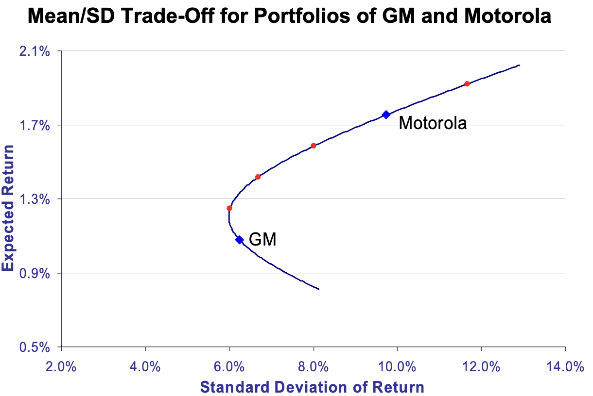
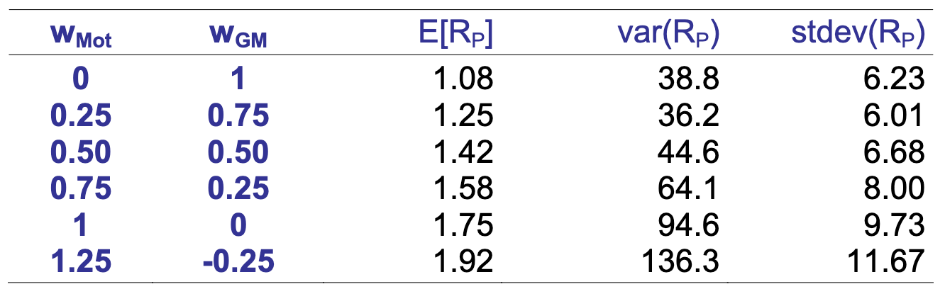
GM and Motorola
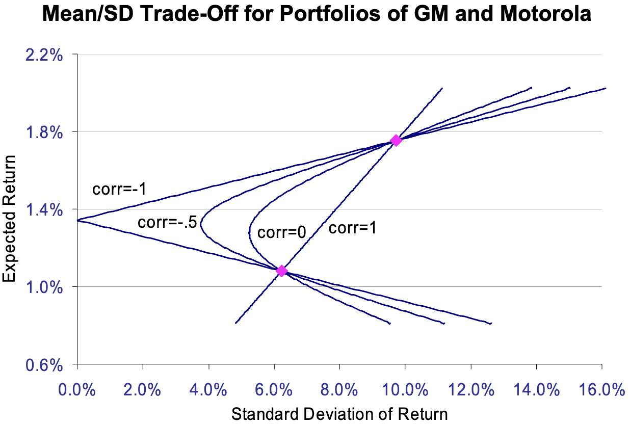
The lecture example uses the following historical monthly moments:
- Motorola mean monthly return: 1.75%, standard deviation: 9.73%
- GM mean monthly return: 1.08%, standard deviation: 6.23%
- Correlation: 0.37
\[ \mathbb{E}[R_p] = w_{\mathrm{GM}}(1.08\%) + w_{\mathrm{MOT}}(1.75\%) \]
\[ \operatorname{Var}(R_p) = w_{\mathrm{GM}}^2\sigma_{\mathrm{GM}}^2 + w_{\mathrm{MOT}}^2\sigma_{\mathrm{MOT}}^2 + 2w_{\mathrm{GM}}w_{\mathrm{MOT}}\operatorname{Cov}(R_{\mathrm{GM}},R_{\mathrm{MOT}}) \]
\[ \operatorname{Var}(R_p) = w_{\mathrm{GM}}^2\sigma_{\mathrm{GM}}^2 + w_{\mathrm{MOT}}^2\sigma_{\mathrm{MOT}}^2 + 2w_{\mathrm{GM}}w_{\mathrm{MOT}}\rho_{\mathrm{GM,MOT}}\sigma_{\mathrm{GM}}\sigma_{\mathrm{MOT}} \]
This shows explicitly that portfolio variance depends on the correlation term as well as on the two stand-alone standard deviations.
What Happens When Correlation Changes?
Suppose the correlation between GM and Motorola changes. What if it
equals
\(-1.0\)?
\(0.0\)?
\(1.0\)?
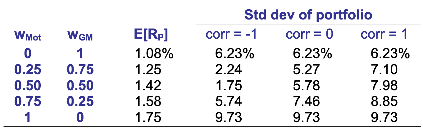
Lower correlation produces lower portfolio standard deviation.
If correlation falls, the feasible set bends further to the left, showing stronger diversification benefits for the same expected return.
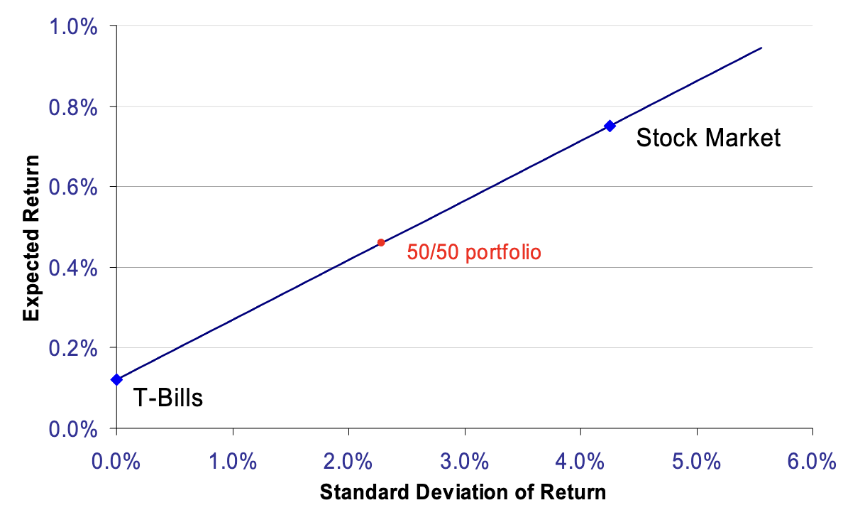
Treasury Bills and the Stock Market
Suppose \(r_f = 0.12\%\) per month and the stock market has \(\mathbb{E}[R_M] = 0.75\%\) and \(\sigma_M = 4.25\%\).
\[ \mathbb{E}[R_p] = w_{\mathrm{TB}}(0.12\%) + w_{\mathrm{STK}}(0.75\%) \]
\[ \operatorname{Var}(R_p) = w_{\mathrm{STK}}^2(4.25\%)^2 \]
These combinations plot on a straight line.
Because Treasury bills are risk free, they contribute no volatility and no covariance, so changing the weight simply moves the investor along a straight capital allocation line in mean--standard deviation space.