How to Measure Risk

Computing Historical Returns

The realized holding-period return on an asset can be written as

\[ R_t = \frac{P_t + D_t - P_{t-1}}{P_{t-1}} \]

where \(P_t\) is the end-of-period price and \(D_t\) is any cash distribution received during the period.

Two basic definitions used throughout the notes are:

\[ \text{Expected return} = \mathbb{E}[R_i], \qquad \text{Excess return} = R_i - r_f \]

Mean, Variance, and Standard Deviation

For a random return \(R_i\),

\[ \mu_i = \mathbb{E}[R_i] \]

\[ \sigma_i^2 = \mathbb{E}\big[(R_i - \mu_i)^2\big] \]

\[ \sigma_i = \sqrt{\sigma_i^2} \]

Sample Estimators

Given a sample of \(T\) realized returns,

\[ \hat{\mu}_i = \frac{1}{T}\sum_{t=1}^{T}R_{i,t} \]

\[ \hat{\sigma}_i^2 = \frac{1}{T-1}\sum_{t=1}^{T}(R_{i,t} - \hat{\mu}_i)^2 \]

If the realized returns are far from their sample mean, the variance is high; in practical terms, the asset is riskier than an investment with a lower variance.

Median

• The median is the 50th percentile, so there is probability one-half that \(R\) lies below it.
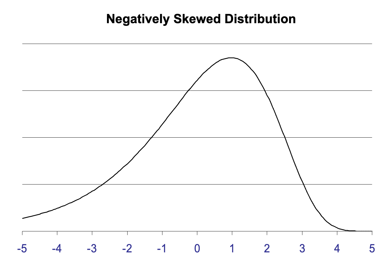
• Skewness
• Skewness captures asymmetry in the return distribution.
• Negative skewness means large losses are more likely than large gains.
• Positive skewness means large gains are more likely than large losses.

Correlation

Correlation asks how closely two random variables move together:

\[ \operatorname{Cov}(R_i,R_j) = \mathbb{E}\big[(R_i-\mu_i)(R_j-\mu_j)\big] \]

\[ \operatorname{Corr}(R_i,R_j) = \frac{\operatorname{Cov}(R_i,R_j)}{\sigma_i \sigma_j} \]