Ennio Alessandrini

01What Regression Analysis Is

Regression analysis is a statistical methodology used to study the relationship between a dependent variable and one or more independent variables.

The dependent variable is the outcome we want to explain or predict (usually denoted by Y). The independent variables are regressors/predictors (X in simple regression, X1, X2, ..., Xk in multiple regression).

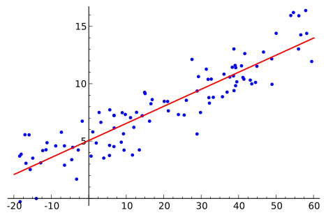
Central question: How does the expected value of Y change when one or more explanatory variables change?

Prediction: estimating future or unknown values of Y from observed X.
Explanation: quantifying direction and magnitude of association.
Inference: testing whether observed relationships are statistically meaningful.
Decision support: guiding economic, business, scientific, and policy choices.

Regression is a formal framework that decomposes observed variation in Y into a systematic component (explained by regressors) and a random component (noise, omitted factors, measurement error).

02The True Population Regression Model

In simple linear regression, the theoretical population model is:

Eq. 1

Y_{i} = β_{0} + β_{1} X_{i} + ε_{i}

Meaning of each term:

Yi: value of dependent variable for observation i.
Xi: value of independent variable for observation i.
beta0: intercept parameter.
beta1: slope parameter.
epsiloni: error term for observation i.

Interpretation of the intercept beta0:

Eq. 2

E (Y ∣ X = 0) = β_{0}

Interpretation of the slope beta1:

Eq. 3

β_{1} = \frac{Δ E ( Y ∣ X )}{Δ X}

The slope effect is constant in simple linear regression: the conditional expectation of Y changes linearly with X.

The error term collects omitted explanatory variables, measurement error, unobserved heterogeneity, random shocks, and model misspecification.

03Conditional Expectation Form of the Model

A formal representation of the regression model is:

Eq. 4

E (Y_{i} ∣ X_{i}) = β_{0} + β_{1} X_{i}

The observed value differs from this conditional mean by the error term:

Eq. 5

Y_{i} = E (Y_{i} ∣ X_{i}) + ε_{i}

Substituting gives the population regression equation:

Eq. 6

Y_{i} = β_{0} + β_{1} X_{i} + ε_{i}

Deterministic part: conditional expectation.
Stochastic part: deviation from conditional expectation.

04Why the True Model Is Unknown

In practice, the whole population is not observed. We observe only a sample:

Eq. 7

(X_{1}, Y_{1}), (X_{2}, Y_{2}), \dots, (X_{n}, Y_{n})

Therefore, population parameters beta0 and beta1 are unknown and must be estimated from sample information.

Estimated regression line:

Eq. 8

\hat{Y}_{i} = \hat{β}_{0} + \hat{β}_{1} X_{i}

beta-hat-0 estimates beta0.
beta-hat-1 estimates beta1.
Y-hat-i is the predicted value for observation i.

05The Least Squares Principle

Ordinary Least Squares (OLS) chooses the fitted line that makes observed points as close as possible to the fitted values.

Residual definition:

Eq. 9

e_{i} = Y_{i} - \hat{Y}_{i}

Eq. 10

e_{i} = Y_{i} - (\hat{β}_{0} + \hat{β}_{1} X_{i})

Scatter plot with fitted regression line and vertical residual segments

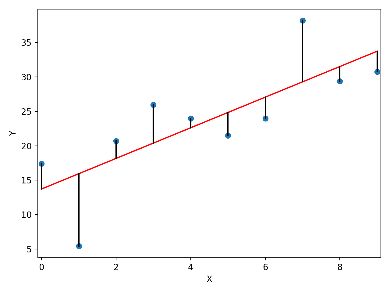
ei > 0: point above fitted line.
ei < 0: point below fitted line.
ei = 0: point on fitted line.

OLS squares residuals to avoid cancellation of positive and negative deviations.

Eq. 11

S S E = i = 1 \sum n e_{i}^{2}

Eq. 12

S S E = i = 1 \sum n (Y_{i} - \hat{Y}_{i})^{2}

Eq. 13

S S E = i = 1 \sum n [Y_{i} - (\hat{β}_{0} + \hat{β}_{1} X_{i})]^{2}

OLS objective: choose beta-hat-0 and beta-hat-1 to minimize total squared residual distance.

Eq. 14

\hat{β}_{0}, \hat{β}_{1} min i = 1 \sum n [Y_{i} - (\hat{β}_{0} + \hat{β}_{1} X_{i})]^{2}

07The Fitted Line and Prediction

After estimating coefficients, the fitted equation is:

Eq. 28

\hat{Y}_{i} = \hat{β}_{0} + \hat{β}_{1} X_{i}

Prediction for a new value X* is:

Eq. 29

\hat{Y}^{*} = \hat{β}_{0} + \hat{β}_{1} X^{*}

The fitted line summarizes the relationship in-sample.
The same equation gives a prediction rule for new X values.

06Derivation of the OLS Estimators

Objective function:

Eq. 15

S (\hat{β}_{0}, \hat{β}_{1}) = i = 1 \sum n [Y_{i} - \hat{β}_{0} - \hat{β}_{1} X_{i}]^{2}

First normal equation (differentiate with respect to intercept):

Eq. 16

\frac{\partial S}{\partial β ^ _{0}} = - 2 i = 1 \sum n (Y_{i} - \hat{β}_{0} - \hat{β}_{1} X_{i})

Eq. 17

i = 1 \sum n (Y_{i} - \hat{β}_{0} - \hat{β}_{1} X_{i}) = 0

Eq. 18

i = 1 \sum n Y_{i} - n \hat{β}_{0} - \hat{β}_{1} i = 1 \sum n X_{i} = 0

Eq. 19

\overset{ˉ}{Y} - \hat{β}_{0} - \hat{β}_{1} \overset{ˉ}{X} = 0

Eq. 20

\hat{β}_{0} = \overset{ˉ}{Y} - \hat{β}_{1} \overset{ˉ}{X}

Second normal equation (differentiate with respect to slope):

Eq. 21

\frac{\partial S}{\partial β ^ _{1}} = - 2 i = 1 \sum n X_{i} (Y_{i} - \hat{β}_{0} - \hat{β}_{1} X_{i})

Eq. 22

i = 1 \sum n X_{i} (Y_{i} - \hat{β}_{0} - \hat{β}_{1} X_{i}) = 0

Eq. 23

\hat{β}_{1} = \frac{\sum _{i = 1}^{n} ( X _{i} - X ˉ ) ( Y _{i} - Y ˉ )}{\sum _{i = 1}^{n} ( X _{i} - X ˉ ) ^{2}}

Eq. 24

i = 1 \sum n (X_{i} - \overset{ˉ}{X}) (Y_{i} - \overset{ˉ}{Y})

Eq. 25

i = 1 \sum n (X_{i} - \overset{ˉ}{X})^{2}

Eq. 26

\hat{β}_{1} = \frac{covariation of X and Y}{variation of X}

Eq. 27

\hat{β}_{0} = \overset{ˉ}{Y} - \hat{β}_{1} \overset{ˉ}{X}

Geometric property: the fitted least-squares line passes through (X-bar, Y-bar).

08Decomposition of Variation: SST, SSR, and SSE

Total variation in Y is decomposed into explained variation and unexplained variation.

Total Sum of Squares (SST):

Eq. 30

S S T = i = 1 \sum n (Y_{i} - \overset{ˉ}{Y})^{2}

Regression Sum of Squares (SSR):

Eq. 31

S S R = i = 1 \sum n (\hat{Y}_{i} - \overset{ˉ}{Y})^{2}

Error Sum of Squares (SSE):

Eq. 32

S S E = i = 1 \sum n (Y_{i} - \hat{Y}_{i})^{2}

Notation used in these three formulas:

$Y_{i}$ observed value of the dependent variable for observation i.

$\hat{Y}_{i}$ fitted or predicted value from the regression line for observation i.

$\overset{ˉ}{Y}$ sample mean of Y.

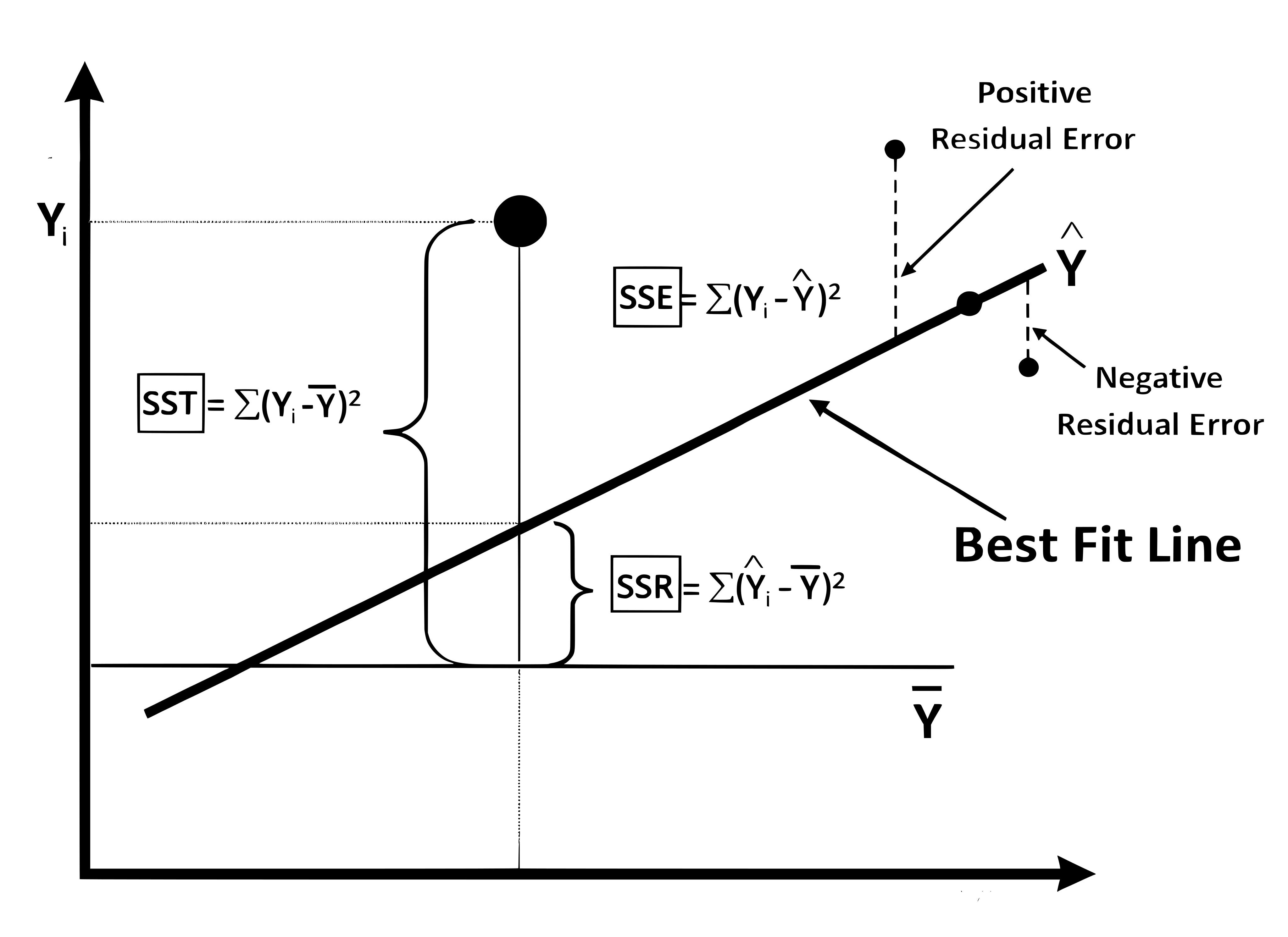
Conceptual variance decomposition visual showing SST, SSR, and SSE around the best fit line

Fundamental identity:

Eq. 33

S S T = S S R + S S E

Total variation = explained variation + unexplained variation.

09Why SST = SSR + SSE

Start from the identity:

Eq. 34

Y_{i} - \overset{ˉ}{Y} = (Y_{i} - \hat{Y}_{i}) + (\hat{Y}_{i} - \overset{ˉ}{Y})

Square both sides:

Eq. 35

(Y_{i} - \overset{ˉ}{Y})^{2} = (Y_{i} - \hat{Y}_{i})^{2} + (\hat{Y}_{i} - \overset{ˉ}{Y})^{2} + 2 (Y_{i} - \hat{Y}_{i}) (\hat{Y}_{i} - \overset{ˉ}{Y})

Sum over all observations:

Eq. 36

i = 1 \sum n (Y_{i} - \overset{ˉ}{Y})^{2} = i = 1 \sum n (Y_{i} - \hat{Y}_{i})^{2} + i = 1 \sum n (\hat{Y}_{i} - \overset{ˉ}{Y})^{2} + 2 i = 1 \sum n (Y_{i} - \hat{Y}_{i}) (\hat{Y}_{i} - \overset{ˉ}{Y})

Under OLS, residuals are orthogonal to fitted values:

Eq. 37

i = 1 \sum n (Y_{i} - \hat{Y}_{i}) (\hat{Y}_{i} - \overset{ˉ}{Y}) = 0

Eq. 38

i = 1 \sum n (Y_{i} - \overset{ˉ}{Y})^{2} = i = 1 \sum n (Y_{i} - \hat{Y}_{i})^{2} + i = 1 \sum n (\hat{Y}_{i} - \overset{ˉ}{Y})^{2}

Eq. 39

S S T = S S E + S S R

10Mean Squared Error and Standard Error of Regression

Mean Squared Error (MSE) in simple regression:

Eq. 40

M S E = \frac{S S E}{n - 2}

In multiple regression with k predictors:

Eq. 41

M S E = \frac{S S E}{n - k - 1}

Standard Error of Regression (SER):

Eq. 42

S E R = M S E

Eq. 43

S E R = \frac{S S E}{n - 2}

Eq. 44

S E R = \frac{S S E}{n - k - 1}

SER measures the typical size of residuals in units of Y: small SER means points are close to the fitted line, large SER means they are more scattered.

Eq. 45

e_{i} = 0 \forall i

Eq. 46

S S E = 0

Eq. 47

M S E = 0

Eq. 48

S E R = 0

11Coefficient of Determination: R^2

R-squared measures the proportion of total variation in Y explained by the regression model.

Eq. 49

R^{2} = \frac{S S R}{S S T}

Eq. 50

R^{2} = 1 - \frac{S S E}{S S T}

Eq. 51

R^{2} = 1 - \frac{\sum _{i = 1}^{n} ( Y _{i} - Y ^ _{i} ) ^{2}}{\sum _{i = 1}^{n} ( Y _{i} - Y ˉ ) ^{2}}

Eq. 52

R^{2} = 0.60

R^2 = 0: model explains none of variation.
R^2 = 1: model explains all variation.
0 < R^2 < 1: partial explanation.
Example: R^2 = 0.60 means 60 percent explained and 40 percent unexplained.

Important caution: high R^2 does not automatically imply causality, correct specification, significant coefficients, or strong out-of-sample performance.

12Adjusted R^2

Ordinary R^2 never decreases when new regressors are added, even if they add little useful information.

Eq. 53

\overset{ˉ}{R}^{2} = 1 - \frac{S S E / ( n - k - 1 )}{S S T / ( n - 1 )}

Eq. 54

\overset{ˉ}{R}^{2} = 1 - (1 - R^{2}) \frac{n - 1}{n - k - 1}

n is sample size.
k is number of predictors.
Adjusted R^2 penalizes unnecessary regressors.
It can increase with useful variables and decrease with weak ones.

Eq. 55

S S E = 0

Eq. 56

R^{2} = 1

If SSE = 0, adjusted R^2 is also 1 because there is no residual error to penalize.

13t-Test for an Individual Coefficient

Beyond estimation, regression supports inference: is the relationship significant, is slope different from zero, and is explanatory power beyond random noise?

For coefficient beta_j, test:

Eq. 57

H_{0} : β_{j} = 0

Eq. 58

H_{1} : β_{j} \neq = 0

Eq. 59

H_{0} : β_{1} = 0

General t-statistic:

Eq. 60

t = \frac{β ^ _{j} - β _{j, 0}}{S E ( β ^ _{j} )}

Eq. 61

t = \frac{β ^ _{j}}{S E ( β ^ _{j} )}

Student t-distribution table diagram for hypothesis testing

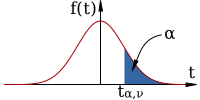
Decision rule based on p-value with residual degrees of freedom (n-2 in simple, n-k-1 in multiple):

Eq. 62

p < α

Eq. 63

∣ t ∣ ≳ 2

Large absolute t suggests stronger evidence against H0; small absolute t suggests weaker evidence.

Reference tableStudent's t Critical Values · Two-Tailed

Select the row corresponding to the appropriate degrees of freedom and the column corresponding to the chosen significance level $α$ .
Reject $H_{0}$ if $∣ t_{calc} ∣ > t^{*}$ .

df	alpha = 0.10	alpha = 0.05	alpha = 0.01
1	6.314	12.706	63.657
2	2.920	4.303	9.925
3	2.353	3.182	5.841
4	2.132	2.776	4.604
5	2.015	2.571	4.032
6	1.943	2.447	3.707
7	1.895	2.365	3.499
8	1.860	2.306	3.355
9	1.833	2.262	3.250
10	1.812	2.228	3.169
12	1.782	2.179	3.055
15	1.753	2.131	2.947
20	1.725	2.086	2.845
25	1.708	2.060	2.787
30	1.697	2.042	2.750
40	1.684	2.021	2.704
60	1.671	2.000	2.660
120	1.658	1.980	2.617
inf	1.645	1.960	2.576

14Standard Error of a Coefficient and F-Statistic

In simple regression, the slope standard error is:

Eq. 64

S E (\hat{β}_{1}) = \frac{S E R ^{2}}{\sum _{i = 1}^{n} ( X _{i} - X ˉ ) ^{2}}

Higher residual noise (SER^2) implies less precision.
Greater variation in X implies more precision.

Overall model significance in multiple regression:

Eq. 65

H_{0} : β_{1} = β_{2} = \dots = β_{k} = 0

Eq. 66

H_{1} : at least one β_{j} \neq = 0

Eq. 67

F = \frac{M S R}{M S E}

Eq. 68

M S R = \frac{S S R}{k}

Eq. 69

M S E = \frac{S S E}{n - k - 1}

Eq. 70

F = \frac{S S R / k}{S S E / ( n - k - 1 )}

Eq. 71

F = \frac{R ^{2} / k}{( 1 - R ^{2} ) / ( n - k - 1 )}

Eq. 72

p < α

Eq. 73

F = t^{2}

In simple regression (one regressor), the overall F-test is equivalent to the t-test on the slope.

15Multiple Regression

Multiple regression model:

Eq. 74

Y_{i} = β_{0} + β_{1} X_{1 i} + β_{2} X_{2 i} + \dots + β_{k} X_{k i} + ε_{i}

Fitted multiple-regression equation:

Eq. 75

\hat{Y}_{i} = \hat{β}_{0} + \hat{β}_{1} X_{1 i} + \hat{β}_{2} X_{2 i} + \dots + \hat{β}_{k} X_{k i}

Each coefficient is interpreted holding all other regressors constant (partial effect).

Example interpretation: beta2 is the expected change in Y for a one-unit increase in X2, keeping other explanatory variables fixed.

Why useful: many outcomes are influenced by several factors simultaneously.

price
advertising
consumer income
seasonal effects
competitor actions

16Overfitting

Overfitting occurs when too many regressors are included relative to the informative structure in data; the model starts capturing random fluctuations instead of systematic relationships.

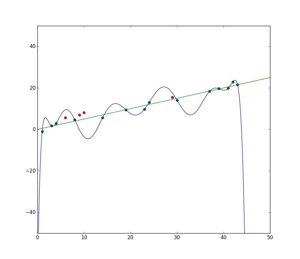
Overfitting regression visual comparing fit complexity

Consequences of overfitting:

very high in-sample R^2
excellent fit on historical data
poor performance on new observations

A strong in-sample fit does not guarantee strong out-of-sample prediction.

Adjusted R^2 helps because it penalizes regressors that do not sufficiently improve explanatory power; unlike ordinary R^2, adjusted R^2 can decrease when complexity is unjustified.

Introduction to Regression Analysis

01What Regression Analysis Is

The Population Regression Model and Its Interpretation