Research objective and question
In this publication, I address a precise operational question:
Did Brexit strengthen or weaken the correlation between the FTSE 100 and the major equity indices of France, Switzerland, Germany, the United States, and Japan?
This is not only a descriptive question. It is a portfolio-strategy question: when correlation changes over time, the quality of international diversification changes as well. The central idea of this work is that a political shock such as Brexit does not generate one linear effect, but a sequence of different regimes.
What I did, operationally
I used daily Bloomberg data for:
FTSE 100(dependent variable)CAC 40,SMI,DAX 40,S&P 500,NIKKEI 225(candidate regressors)
Sample horizon:
- market data:
02/01/2014 - 31/05/2024 - final rolling series:
01/05/2014 - 31/05/2024
Estimation structure:
- rolling window length:
86observations - total rolling regressions:
2632
This architecture was chosen for one specific reason: avoiding a single full-sample "average" regression that hides structural change, and observing instead how the FTSE-external-market relationship evolves day by day.
Why not a single static model
A static 10-year model would be too rigid relative to events such as:
- Brexit referendum (
23/06/2016) - official UK exit from the EU (
31/01/2020) - pandemic shock and the post-2023 phase
For this reason, the methodology was built around:
- rolling coefficient estimation
- continuous comparison between reduced and full models
- daily best-model selection through F-testing
- dynamic analysis of the selected model's
Key econometric steps
Below I keep only the central formulas of the empirical exercise, i.e., those required to run the estimation and make model-selection decisions.
1) Rolling regression with time-varying parameters
2) OLS estimation in each window
3) Full model and baseline model
Full model:
Baseline model (from the preliminary forward phase):
4) Unrestricted vs restricted model comparison
For each window I computed:
with joint test:
5) F-statistic used in model selection
I then defined a decision dummy:
and the average rejection rate over all 2632 windows:
In the final results this frequency is approximately 19.41%.
6) Turning-point detection
To distinguish strengthening/weakening regimes I compared 10-day and 60-day moving averages:
Using one-sided thresholds -2.39 and +2.39 (58 d.f., ).
Selection logic implemented (detailed)
The "modified stepwise backward" procedure does not remove variables once in a static way; it does so day by day inside each rolling window.
Order of candidate models compared:
CAC + SWISSCAC + SWISS + S&PCAC + SWISS + DAXCAC + SWISS + NIKKEICAC + SWISS + S&P + DAXCAC + SWISS + S&P + NIKKEICAC + SWISS + DAX + NIKKEICAC + SWISS + S&P + DAX + NIKKEI
Applied decision rule:
- if the reduced model is not rejected against the full model, keep the reduced model
- if multiple models are admissible within the same block, keep the one with the best
- store that selected model's as the daily value of the final series
This is the core contribution of the exercise: the analysis is not estimating one "average" correlation, but a selected and time-updated correlation structure based on statistical testing.
Main empirical results
Selection frequencies over 2632 days:
| Selected model | Count | Relative frequency |
|---|---|---|
| CAC + SWISS | 2121 | 0.8059 |
| CAC + SWISS + S&P | 281 | 0.1068 |
| CAC + SWISS + DAX | 126 | 0.0479 |
| CAC + SWISS + NIKKEI | 51 | 0.0194 |
| CAC + SWISS + S&P + DAX | 40 | 0.0152 |
| CAC + SWISS + S&P + NIKKEI | 9 | 0.0034 |
| CAC + SWISS + DAX + NIKKEI | 4 | 0.0015 |
| Full model (5 regressors) | 0 | 0.0000 |
Structural summary:
- 2-variable models:
80.59% - 3-variable models:
17.40% - 4-variable models:
2.01% - full model:
0%
Interpretation: FTSE dependence remains mainly Eurocentric (CAC-SWISS), while additional regressors enter only episodically and in a regime-dependent way.
Rolling R2 and regime reading
Rolling R2 and models selected each day (data from 01/05/2014 to 31/05/2024)
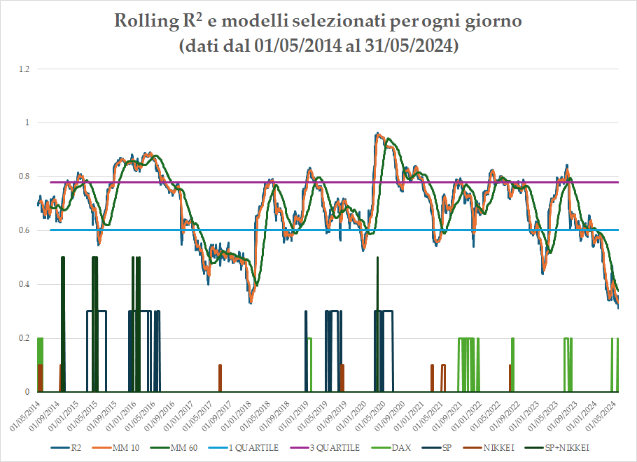
Sample references used in the chart:
Q1 = 0.6029Q3 = 0.7788- observed range: approximately
0.30 - 0.90
Argument-based phase reading:
- Post referendum (2016-2018): persistent downward path and progressive decorrelation.
- 2018-early 2020: return to interquartile range and stabilization.
- 2020-2021: correlation peak during systemic global shock.
- 09/2023-05/2024: new weakening phase with recent lows.
The results chapter identifies 38 turning points, consistent with non-linear dynamics and multiple regime changes.
What this work demonstrates, in substance
The strongest conclusion is not simply "Brexit increases" or "Brexit decreases" correlation in absolute terms. The strongest conclusion is both methodological and economic:
- the FTSE-external-market relationship is time-varying
- Brexit acts as a shock that initiates a first decorrelation phase
- subsequent global shocks (COVID, geopolitical context) temporarily re-synchronize correlations
- in the last sample segment, a renewed weakening of co-movement emerges
Conclusion
This analysis answers the research question with a non-simplistic conclusion: the Brexit effect is mixed and dynamic. The rolling procedure with F-test-based model selection is what makes the result robust, because it translates historical change into a statistically traceable day-by-day sequence.